
Plots the wildfire greenhouse gas emissions data retrieved using get_fires_emissions() with ggplot2.
The output ggplot2 object may be further modified.
Usage
plot_fires_emissions(
  dataset = get_fires_emissions(),
  pollutant = c("CO2", "BC", "C", "CH4", "CO", "NMHC", "NOX", "OC", "PM2.5", "SO2", "TC"),
  style = c("cumulative", "weekly"),
  print = TRUE
)
Arguments
- dataset
Name of the tibble generated by
get_fires_emissions- pollutant
(string) Select which pollutant to plot. May be one of
"CO2"(the default),"BC","C","CH4","CO","NMHC","NOX","OC","PM2.5","SO2", or"TC".- style
(string) Select cumulative or weekly view. May be
"cumulative"(year-to-date totals, the default) or"weekly"(weekly values).(boolean) Display the ggplot2 chart, defaults to TRUE. Use FALSE to suppress display.
Details
plot_fires_emissions invisibly returns a ggplot2 object with a pre-defined wildfire
emissions chart using data from get_fires_emissions. By default the chart is also displayed.
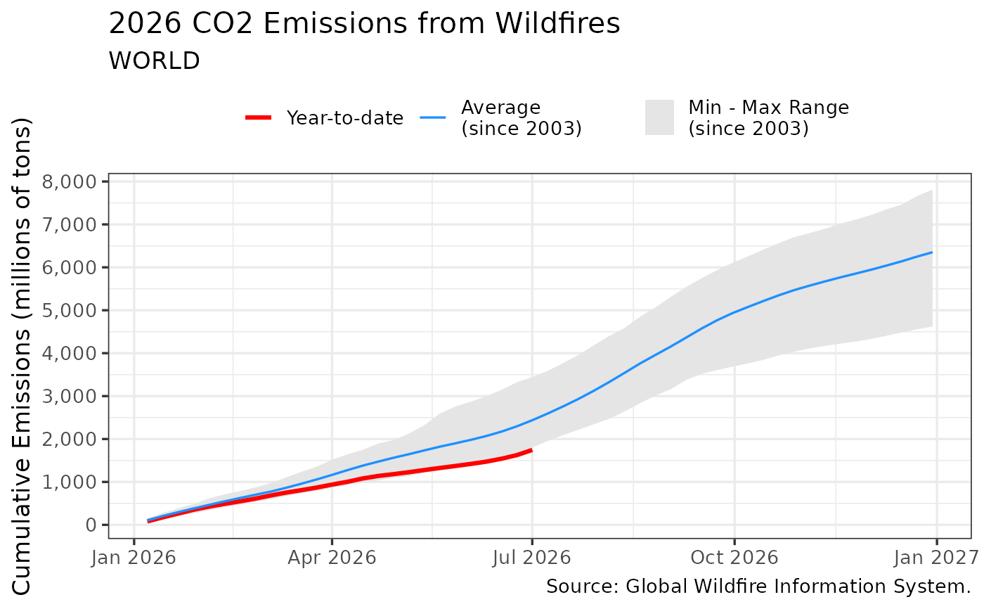
The shaded ribbon shows the historical minimum-to-maximum range since 2003, and the blue line
shows the historical average. Emissions are expressed in millions of tons. Users may further
modify the output ggplot2 chart.
Author
Hernando Cortina, hch@alum.mit.edu
Examples
# \donttest{
# Fetch wildfire emissions data:
emissions <- get_fires_emissions()
#
# Plot output using package's built-in ggplot2 defaults
plot_fires_emissions(emissions)
 # Or just call plot_fires_emissions(), which defaults to get_fires_emissions() dataset
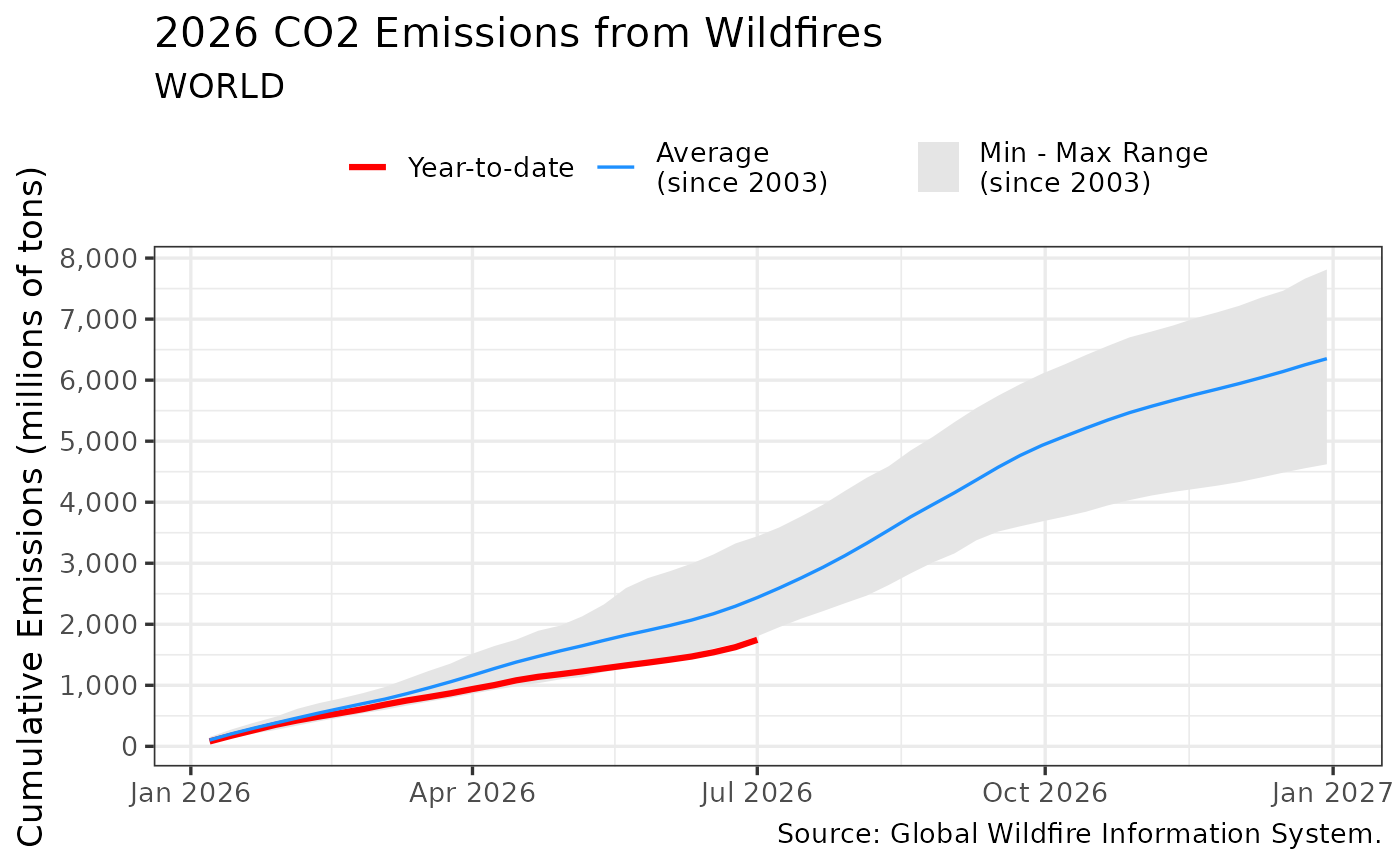
plot_fires_emissions()
# Or just call plot_fires_emissions(), which defaults to get_fires_emissions() dataset
plot_fires_emissions()
 # Plot weekly PM2.5 emissions instead of cumulative CO2
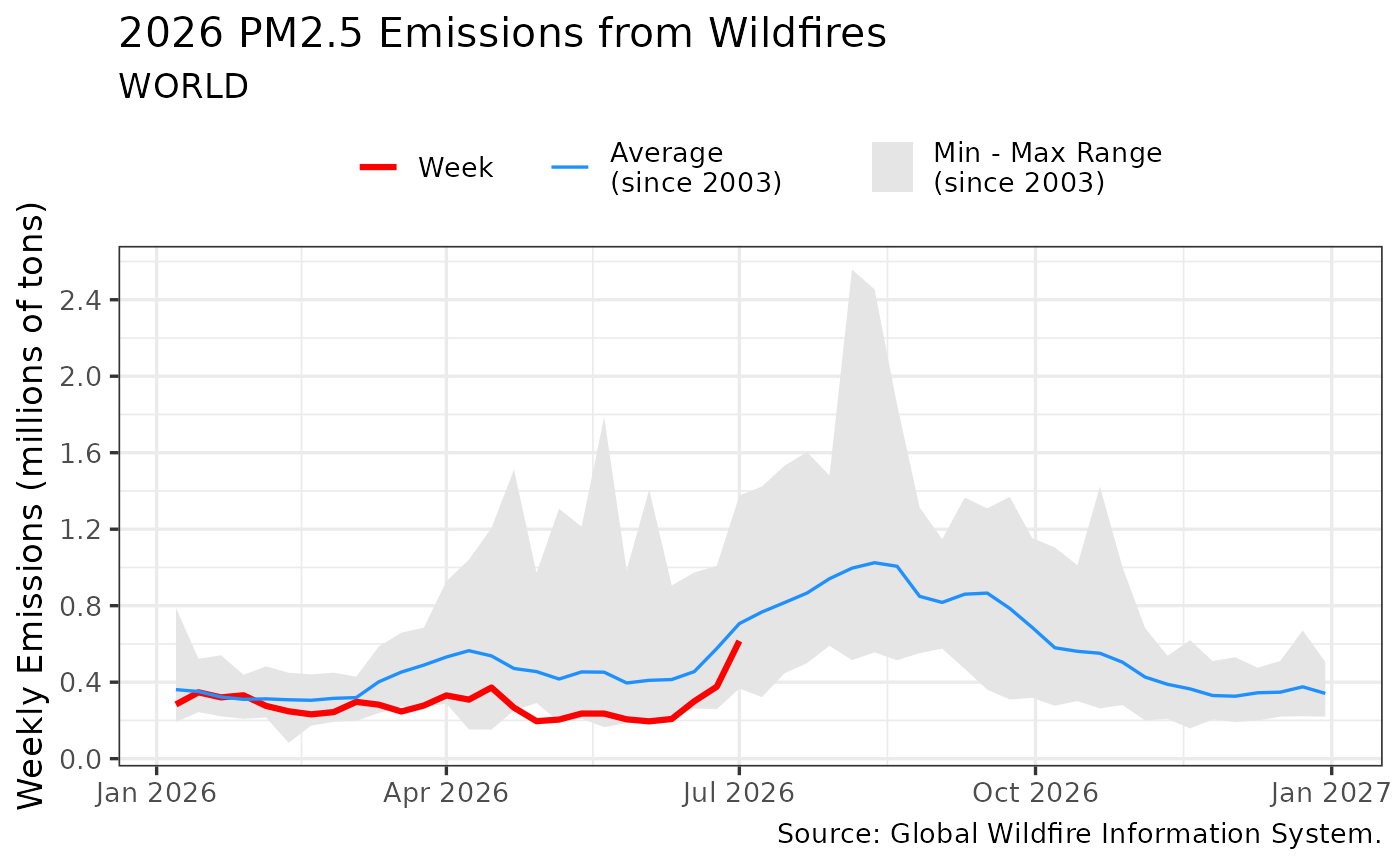
plot_fires_emissions(emissions, pollutant = 'PM2.5', style = 'weekly')
# Plot weekly PM2.5 emissions instead of cumulative CO2
plot_fires_emissions(emissions, pollutant = 'PM2.5', style = 'weekly')
 p <- plot_fires_emissions(emissions, print = FALSE)
# Modify plot such as: p + ggplot2::labs(title='Global CO2 Emissions from Wildfires') # }
p <- plot_fires_emissions(emissions, print = FALSE)
# Modify plot such as: p + ggplot2::labs(title='Global CO2 Emissions from Wildfires') # }