
Plots the wildfire burnt area or fire count data retrieved using get_fires_area() with ggplot2.
The output ggplot2 object may be further modified.
Usage
plot_fires_area(
  dataset = get_fires_area(),
  var = c("area", "count"),
  style = c("cumulative", "weekly"),
  print = TRUE
)
Arguments
- dataset
Name of the tibble generated by
get_fires_area- var
(string) Select which variable to plot. May be
"area"(burnt area in hectares, the default) or"count"(number of fire events).- style
(string) Select cumulative or weekly view. May be
"cumulative"(year-to-date totals, the default) or"weekly"(weekly values).(boolean) Display the ggplot2 chart, defaults to TRUE. Use FALSE to suppress display.
Details
plot_fires_area invisibly returns a ggplot2 object with a pre-defined wildfire chart using
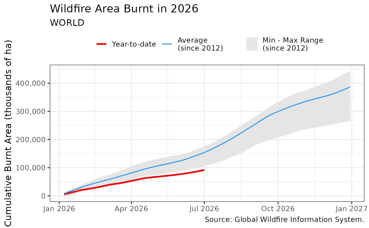
data from get_fires_area. By default the chart is also displayed. The shaded ribbon shows the
historical minimum-to-maximum range since 2012, and the blue line shows the historical average.
Users may further modify the output ggplot2 chart.
Author
Hernando Cortina, hch@alum.mit.edu
Examples
# \donttest{
# Fetch wildfire data:
fires <- get_fires_area()
#
# Plot output using package's built-in ggplot2 defaults
plot_fires_area(fires)
 # Or just call plot_fires_area(), which defaults to get_fires_area() dataset
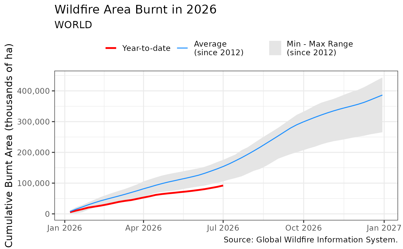
plot_fires_area()
# Or just call plot_fires_area(), which defaults to get_fires_area() dataset
plot_fires_area()
 # Plot weekly fire count instead of cumulative burnt area
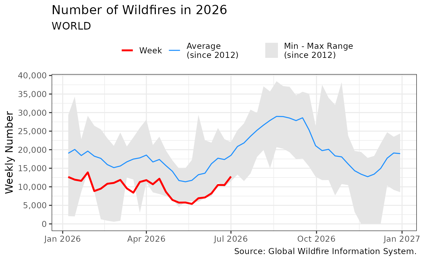
plot_fires_area(fires, var = 'count', style = 'weekly')
# Plot weekly fire count instead of cumulative burnt area
plot_fires_area(fires, var = 'count', style = 'weekly')
 p <- plot_fires_area(fires, print = FALSE)
# Modify plot such as: p + ggplot2::labs(title='Global Wildfire Burnt Area') # }
p <- plot_fires_area(fires, print = FALSE)
# Modify plot such as: p + ggplot2::labs(title='Global Wildfire Burnt Area') # }